Linear Functions
Contents
Linearity
Linear functions describe functions that preserve both additivity and scalar multiplication.
To break this jargon down:
- Additivity: Property of a function where the following holds true: f(u + v) = f(u) + f(v)
- Scalar multiplication: Property of a function where the following holds true: f(cu) = cf(u)
To think about this much more easily, Linear Functions are functions where the input variable has a degree (that is, exponent value) of 1 (like f(x)=2x + 2) or 0 (like f(x)=2).
Types
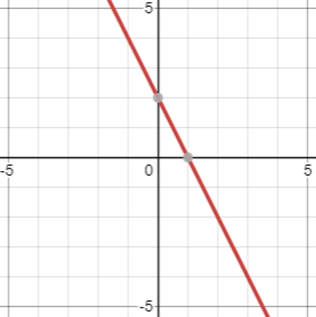
Linear functions present themselves like the following chart. Notice that the graph is just a line (hence, LINEar)
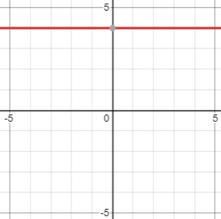
Constant functions are a special type of linear function where, for all output, the output is the same value. These are of the form f(x) = c, where c simply represents some numerical value.
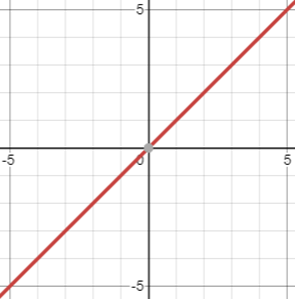
Identity: A special type of linear function where the output is the same as the input. It is of the form, f(x) = x.
Forms
Linear functions have important characteristics beyond the preservation of additivity and scalar multiplication.
Linear functions are typically of the form:
y = mx + b
Where y is the output variable (could be f(x), g(x), z, etc.), x is the input variable, and:
-
Slope (m): The number describing the direction and steepness of the function’s behavior.
- Also known as rate of change.
- A function’s steepness is given by the magnitude of the slope (that is, how big).
- A function’s direction is given by the sign of the slope. That is:
- A positive slope (m > 0) means the output grows as the input grows.
- A negative slope (m < 0) means the output shrinks (“grows” more negative) as the input grows larger.
- A slope of zero (m=0) means the output remains the same no matter the input. That is, this is a constant function!
-
Intercept (b): The constant number which essentially provides a shift of the function’s values.
- This may also be thought of as the “default” value for y, which is the value of y when x=0. This is known as the y-intercept.
For this reason, the form, y=mx+b is known as slope-intercept form since it describes both the slope and the intercept of a single function.
Another form that may be utilized is the point-slope form, which enables defining a function utilizing two ordered pairs.
y - y_1 = m(x-x_1)
The first pair is going to be (x, y), as you are defining the behavior between x and y. The second pair will be ANY point on the line, represented by (x_1, y_1).
Point-slope form may always be simplified into slope-intercept form, and slope-intercept form may always be expanded into point-slope form (so long as the point chosen resides on the line).
Example:
y - 3 = 2(x-4)
y - 3 = 2x - 2(4)
y - 3 = 2x - 8
\boxed{y = 2x - 5}
Point-slope form is converted to slope-intercept by solving for y!
Slope-intercept form is more open-ended, since you may chose any point. You simply extract the slope and choose a point on the line. For instance: y = f(x) = 2x - 5.
Say we choose to utilize x_1=12.
First, solve for f(12): y = f(12) = 2(12) - 5 = 24 - 5 = \boxed{19}
This is your (x_1, y_1) ordered pair. Now, we know that the original slope is 2 (since, in slope intercept form, we have y = \underline{2}x - 5). Plug this into the point-slope form template:
y - y_1 = m(x - x_1)
y - 19 = 2(x - 12)
To confirm there are no more mistakes, you can convert it back to slope intercept form, to ensure that the original form is the same as this new form!
y - 19 = 2(x - 12)
y - 19 = 2x - 24
\boxed{y = 2x - 5} \; \checkmark
Closing
| Previous | Next |
|---|---|
| ← 1.3.0 | 1.3.2: Forms → |